Pipeline Management

You've got reps entering 75% probabilities on deals with a 15% chance of closing. You've got pipeline reviews where "gut feel" masquerades as insight. And you've got executives making resource decisions based on numbers that bear no resemblance to reality.

The cost? Missed quarters. Blown capacity plans. Sales comp payouts that reward luck over skill. And a permanent credibility gap between what sales says will happen and what actually does.

If you're serious about forecast accuracy and revenue predictability, you need to replace intuition with data science. That's where probability modeling comes in.

What is Probability Modeling?

Probability modeling applies statistical methods to calculate the likelihood that a specific opportunity will close. Rather than relying on sales rep judgment or fixed stage percentages, probability models analyze multiple data points—deal characteristics, behavioral signals, historical patterns—to generate empirically-grounded predictions.

The goal isn't perfect prediction. That's impossible. The goal is to consistently outperform human judgment at scale, providing forecast accuracy that compounds into better planning, resource allocation, and strategic decisions.

Why Traditional Approaches Fail

Most organizations start with simple stage-based probability:

Discovery: 10%
Qualification: 25%
Proposal: 50%
Negotiation: 75%
Closed Won: 100%

This approach has exactly one advantage: it's easy to implement. But it has many disadvantages.

It ignores deal-specific factors. A $10K deal in Negotiation has wildly different close probability than a $1M deal in the same stage. Stage alone explains maybe 30-40% of variance in close outcomes.

It assumes linear progression. Deals don't move uniformly through stages. Some jump from Discovery to Negotiation. Others ping-pong between Proposal and Qualification for months. Static stage probabilities can't capture this complexity.

It encourages gaming. When probabilities are fixed by stage, reps learn to manipulate stage progression to hit forecast targets. The data becomes polluted by strategic stage changes rather than actual deal progression.

It provides no feedback loop. Because probabilities are fixed, there's no mechanism to learn from outcomes and improve predictions over time.

Advanced probability modeling addresses these limitations.

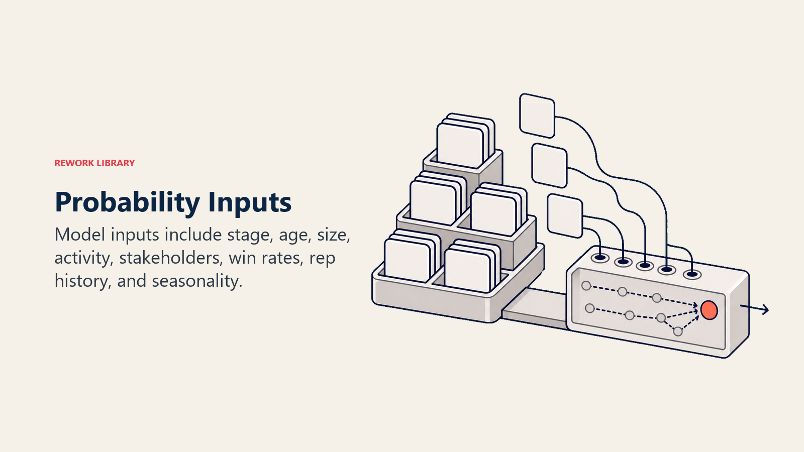
Probability Inputs and Factors

Good probability models incorporate multiple signal categories:

1. Pipeline Stage

Stage remains relevant—it captures progression through a defined sales process—but it's one factor among many rather than the sole determinant.

What matters is measuring actual stage exit rates from your historical data, not using industry averages or aspirational targets. If your "Negotiation" stage historically closes at 42%, that's your baseline. Not 75%.

2. Deal Age

Time since opportunity creation or stage entry correlates strongly with close probability. Deals that linger in stages beyond typical cycle times show declining win rates.

Good models track absolute age (days since opportunity creation), stage age (days in current stage), and expected versus actual velocity (deviation from historical norms).

A deal that's been in Proposal for 90 days when your median is 14 days? Probability should reflect that reality.

3. Deal Size

Deal value influences close probability in non-linear ways. Very small deals may have lower qualification rigor, leading to higher disqualification rates. Very large deals face longer cycles, more stakeholders, and heightened scrutiny.

The relationship varies by your business model, average contract value, and deal size distribution. The model learns these patterns from historical outcomes.

4. Activity Patterns

Meeting frequency, email engagement, call volume, and demo completion all signal deal health. But raw activity counts matter less than patterns: Is engagement increasing or decreasing? Are you reaching decision-makers? Are prospects initiating contact? Are follow-up actions being completed?

Models that incorporate activity signals typically improve accuracy by 15-25% over stage-only approaches.

5. Stakeholder Engagement

B2B deals require consensus across multiple stakeholders. Models that factor in contact role diversity, champion identification, and decision-maker engagement consistently outperform those that don't.

Key signals include number of contacts logged, roles represented (economic buyer, technical evaluator, champion), executive engagement level, and committee versus single decision-maker dynamics.

6. Historical Win Rates

The most predictive factor is often similarity to past closed deals. Models can compare current opportunities against historical cohorts based on:

Industry/vertical match
Company size segment
Product/solution type
Competition encountered
Source channel

If deals from a specific lead source historically close at 18%, new opportunities from that source should inherit that baseline, adjusted for other factors.

7. Sales Rep Performance

Individual rep win rates vary significantly. A model that incorporates rep-level historical performance—while accounting for territory quality and sample size—produces more accurate forecasts than one that treats all reps identically.

This isn't about blaming underperformers. It's about accurately weighting each opportunity based on all available information, including who's running the deal.

8. Seasonal and Temporal Factors

Many businesses exhibit seasonal patterns:

Budget flush in Q4
Slow summer months
End-of-quarter urgency
Fiscal year-end dynamics

Models can incorporate these temporal effects, adjusting probabilities based on close date timing and historical seasonal conversion patterns.

Probability Modeling Approaches

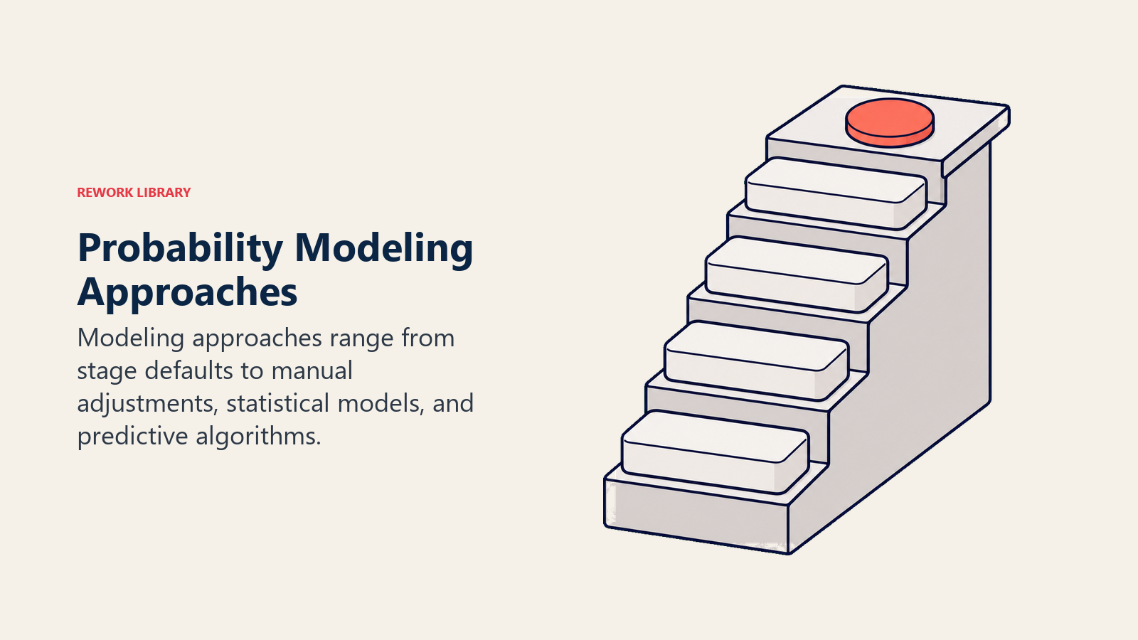
Organizations typically progress through several modeling sophistication levels:

Simple: Stage-Based Only

How it works: Fixed percentages assigned to each pipeline stage.

Pros: Easy to implement, universally understood, requires no data science.

Cons: Ignores deal-specific factors, encourages gaming, no learning mechanism.

Typical accuracy: 40-60% of deals close within 10 percentage points of predicted probability.

Best for: Early-stage companies with limited historical data (<100 closed deals).

Intermediate: Stage + Manual Adjustment

How it works: Stage provides baseline probability. Reps adjust based on their judgment of deal quality.

Pros: Incorporates rep knowledge, flexible for unique situations.

Cons: Highly subjective, prone to optimism bias, difficult to audit or improve.

Typical accuracy: 45-65% within 10 percentage points. Improvement over stage-only is marginal because biases persist.

Best for: Small teams where rep judgment is well-calibrated and management can spot-check adjustments.

Advanced: Multi-Factor Statistical Models

How it works: Logistic regression or similar statistical techniques analyze historical outcomes to weight multiple factors (stage, age, size, activities, etc.) and calculate probability scores.

Pros: Data-driven, incorporates multiple signals, improves over time as more outcomes accumulate, auditable.

Cons: Requires sufficient historical data (500+ closed opportunities), needs periodic retraining, less intuitive for sales teams.

Typical accuracy: 65-80% within 10 percentage points, with continuous improvement.

Best for: Growth-stage and enterprise companies with mature CRM hygiene and enough historical data.

AI/ML: Predictive Algorithms

How it works: Machine learning algorithms (random forests, gradient boosted trees, neural networks) identify complex, non-linear relationships across dozens or hundreds of features.

Pros: Captures subtle patterns invisible to human analysts, handles feature interactions, provides highest accuracy.

Cons: Requires large datasets (2,000+ closed opportunities), black-box nature complicates explanation, demands ML expertise or platform investment.

Typical accuracy: 75-85% within 10 percentage points at mature deployment.

Best for: Enterprise organizations with robust data infrastructure, ML capabilities, and high-value deals where accuracy improvements justify investment.

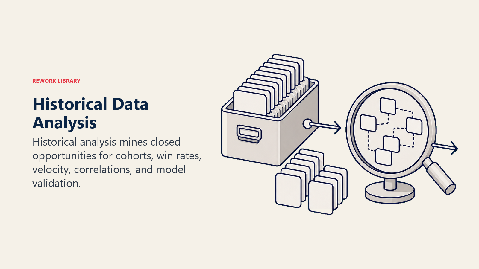
Historical Data Analysis

Building an effective probability model requires mining your historical deal data for patterns. This isn't a one-time exercise—it's an ongoing practice.

Data Requirements

Minimum viable dataset:

500+ closed opportunities (won + lost)
12+ months of history
Clean stage progression tracking
Consistent opportunity creation practices
Basic activity logging

For advanced models:

2,000+ closed opportunities
24+ months of history
Detailed activity logs (meetings, emails, calls)
Contact role data
Product/service detail
Competitive intelligence

Analytical Process

1. Cohort definition: Segment historical opportunities by relevant dimensions (deal size bands, verticals, products, rep tenure, lead source).

2. Win rate calculation: Calculate actual close rates for each cohort at each stage. This becomes your empirical baseline, replacing generic percentages.

3. Velocity analysis: Measure median and distribution of stage durations and total cycle time. Deals that deviate significantly from these norms warrant probability adjustments.

4. Feature correlation: Identify which factors correlate most strongly with closed-won outcomes. Not all signals matter equally. Focus model complexity on high-signal factors.

5. Model training: Use historical data to train statistical or ML models. Split data into training (70%), validation (15%), and test sets (15%) to avoid overfitting.

6. Accuracy testing: Measure model performance on hold-out test data. Key metrics include calibration (do 60% probabilities actually close 60% of the time?) and discrimination (can the model separate winners from losers?).

Cohort-Based Modeling

One powerful modeling approach groups similar opportunities into cohorts and applies cohort-specific conversion rates.

Defining Meaningful Cohorts

Effective cohorts balance specificity (narrow enough to be predictive) with sample size (large enough for statistical significance).

Examples:

Deal size + stage: "$50-100K opportunities in Proposal"
Industry + product: "Healthcare deals for compliance solution"
Source + stage: "Inbound demo requests in Discovery"
Rep segment + size: "Enterprise AEs with $200K+ deals"

The goal is creating groups where internal variance in close rates is low and between-group variance is high. Statistical techniques like decision trees naturally identify these splits.

Applying Cohort Probabilities

Once cohorts are defined with historical close rates, new opportunities are assigned to the appropriate cohort and inherit that baseline probability.

Example: A $75K deal in Proposal stage from an inbound source might match the "$50-100K, Proposal, Inbound" cohort with a 47% historical close rate. That becomes the starting probability, potentially adjusted by other real-time factors.

Dynamic Cohort Membership

As deals progress, they move between cohorts. A deal that advances from Proposal to Negotiation shifts to a new cohort with a different baseline probability. Stage changes thus affect probability—but based on empirical data rather than fixed assumptions.

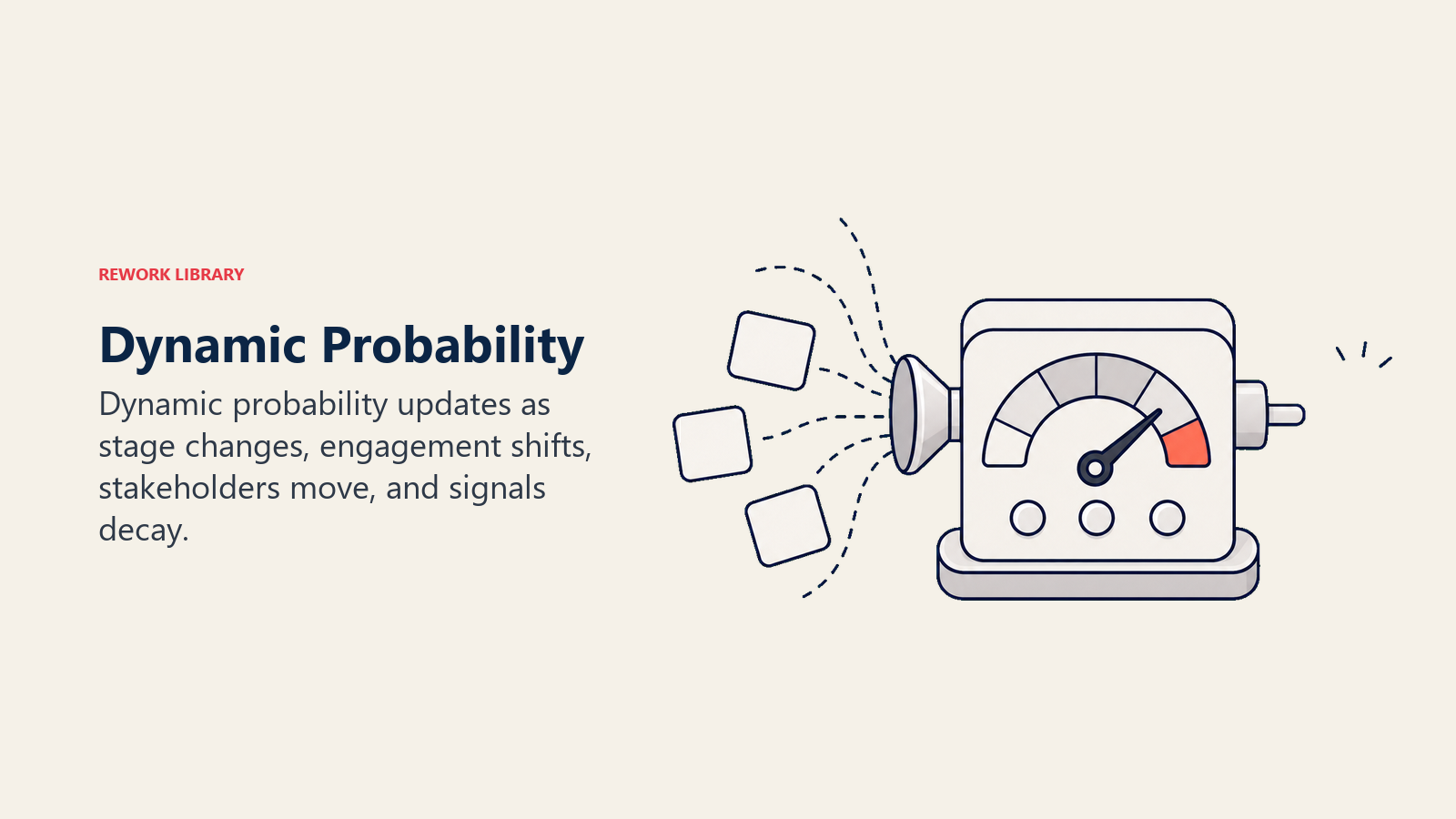
Dynamic Probability

The most sophisticated models treat probability as a continuously updating value that responds to new signals in real-time.

Trigger-Based Adjustments

Specific events trigger probability recalculations:

Stage progression: Advancing or regressing stages
Activity spikes or gaps: Sudden increase in engagement or radio silence
Stakeholder changes: New champion identified or key contact exits
Time decay: Deal aging beyond expected velocity
Close date shifts: Pushing expected close date forward

Each trigger feeds into the model, which recalculates probability incorporating the new information.

Bayesian Updating

A Bayesian approach starts with a prior probability (based on cohort or initial factors) and updates it as evidence accumulates. Each new data point—a completed meeting, a sent proposal, a week of inactivity—updates the posterior probability estimate.

This approach elegantly handles uncertainty and incorporates information asymmetrically: strong positive signals increase probability more than weak signals, and disconfirming evidence appropriately reduces estimates.

Signal Decay

Not all data points carry equal weight over time. A demo conducted 90 days ago is less predictive than one completed last week. Dynamic models can decay the influence of older signals while emphasizing recent engagement.

This prevents stale data from artificially inflating or suppressing probabilities on deals where circumstances have changed.

Probability Overrides

Even the best model will occasionally misread a situation that the rep understands better. Override mechanisms provide necessary flexibility while maintaining auditability.

When Overrides Make Sense

Legitimate override scenarios:

Unique deal circumstances: Merger, acquisition, or leadership change affecting timeline
External information: Competitive loss or unexpected budget approval not captured in CRM
Relationship insights: Personal relationship with decision-maker providing confidence the model can't see
Process deviations: Deal following non-standard path (e.g., executive-led fast track)

Override Governance

Uncontrolled overrides defeat the purpose of modeling. Effective governance includes:

Requiring justification: Reps must document why they're overriding and what information justifies the change.

Limiting magnitude: Caps on override size (e.g., ±20 percentage points) prevent wholesale replacement of model predictions.

Tracking accuracy: Monitor whether overridden deals close at overridden probabilities or model probabilities. If reps consistently override downward and deals still close, that's useful feedback. If they override upward and deals consistently miss, that's coaching opportunity.

Approval thresholds: Large overrides or overrides on high-value deals may require manager approval.

Feedback loops: Override outcomes feed back into model training. If reps repeatedly override for similar reasons and prove correct, that signal should be incorporated into the model.

Model Validation

Building a model is easy. Building an accurate model that improves over time requires rigorous validation.

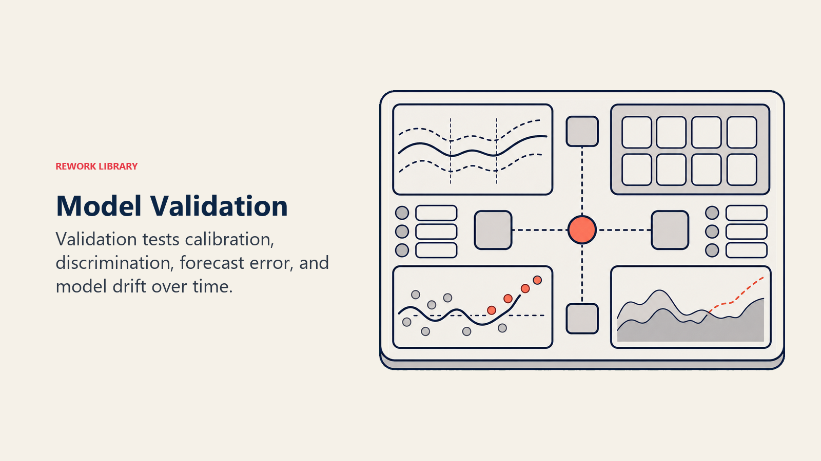
Calibration Testing

A well-calibrated model assigns probabilities that match actual outcomes across probability bands.

Test: Group historical opportunities by predicted probability bands (0-10%, 10-20%, ..., 90-100%). Calculate actual close rates within each band. A calibrated model shows close alignment.

Example:

Predicted 50-60% probability → Actual 48% closed (well-calibrated)
Predicted 70-80% probability → Actual 58% closed (overconfident)

Poor calibration indicates systematic bias requiring model retraining or feature engineering.

Discrimination Analysis

Discrimination measures the model's ability to separate deals that close from those that don't.

Key metrics:

AUC-ROC: Area Under Receiver Operating Characteristic curve. Values above 0.75 indicate good discrimination, above 0.85 excellent.
Precision-Recall: At what predicted probability threshold does the model correctly identify closeable deals without excessive false positives?

High discrimination means the model isn't just well-calibrated on average—it's actually sorting opportunities by true close likelihood.

Forecast Error Analysis

The ultimate test: does the model improve weighted pipeline forecast accuracy?

Compare:

Predicted total weighted pipeline (sum of opportunity values × probabilities)
Actual closed revenue over forecast period

Calculate mean absolute percentage error (MAPE) and compare against previous forecasting approaches. A good model should reduce MAPE by 20-40% versus stage-based forecasting.

Ongoing Monitoring

Model performance degrades over time as:

Business conditions change
Product/market fit evolves
Sales processes mature
Team composition shifts

Implement quarterly model reviews examining:

Recent calibration and discrimination metrics
Forecast error trends
Feature importance drift (are factors that mattered six months ago still predictive?)
Cohort stability (have historical close rates shifted?)

Retrain models when performance degrades or annually at minimum.

Implementation

Successfully deploying probability modeling requires addressing technology, process, and change management.

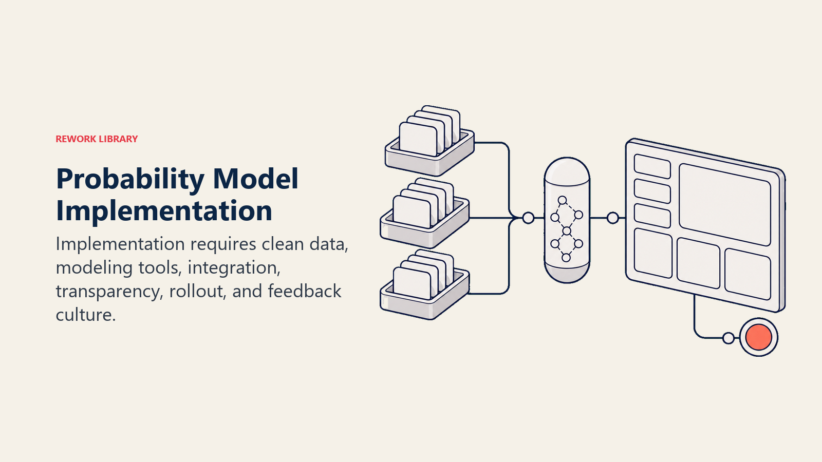
Technology Requirements

Data infrastructure: Clean, centralized CRM data with consistent opportunity tracking, stage definitions, and activity logging. Garbage data in = garbage predictions out.

Modeling platform: Options range from:

CRM-native: Salesforce Einstein, Microsoft Dynamics Insights
Specialized sales analytics: Clari, Gong Forecast, People.ai
Custom models: Python/R models deployed via API to CRM

Choice depends on data volume, modeling sophistication required, and in-house data science capability.

Integration architecture: Models must integrate with existing tools—CRM, stage-based forecasting dashboards, reporting systems—to provide predictions where teams already work.

Change Management

Probability modeling fails more often due to adoption issues than technical problems.

Executive sponsorship: RevOps or sales leadership must champion the model, explain the "why," and commit to using model outputs in decision-making.

Transparency: Share how the model works, what factors it considers, and why it outperforms gut feel. Black-box systems breed distrust.

Gradual rollout: Start with reporting mode (showing model predictions alongside existing probabilities) before making model outputs authoritative. This builds trust and identifies edge cases.

Training: Sales teams need to understand what behaviors improve deal probability (stakeholder expansion, consistent activity, velocity maintenance) versus what doesn't affect model predictions (wishful thinking, sandbagging).

Incentive alignment: If comp plans still reward forecast accuracy based on rep-entered probabilities, reps will game the system. Align incentives with model adoption.

Feedback Culture

The best models improve continuously because organizations treat prediction errors as learning opportunities.

After every quarter:

Review deals that closed despite low predicted probability (what signals did the model miss?)
Review deals that missed despite high predicted probability (what warning signs were ignored?)
Update cohort definitions and feature sets based on findings
Retrain models incorporating latest outcomes

This flywheel—prediction, outcome observation, analysis, model improvement—compounds into increasing forecast accuracy over time.

The Competitive Advantage of Probability Modeling

Organizations that master probability modeling gain compounding advantages:

Resource allocation: Invest coaching time, sales engineering support, and executive involvement in high-probability opportunities rather than spreading resources evenly.

Pipeline management: Identify at-risk deals early based on probability decay, enabling proactive intervention rather than surprised quarter-end misses.

Capacity planning: Accurate weighted pipeline enables better hiring, quota setting, and territory design decisions.

Strategic clarity: When forecasts consistently match outcomes, leadership can make growth investments, product decisions, and market expansion choices with confidence rather than hedging against forecast volatility.

Most importantly, probability modeling shifts the conversation from arguing about deal quality to diagnosing why certain deal patterns succeed and others fail—enabling systematic improvement rather than perpetual hope.

Conclusion: From Gut-Feel to Data Science

Sales will always retain elements of art—relationship building, negotiation nuance, reading room dynamics. But forecasting shouldn't be art. It should be science.

Probability modeling transforms forecasting from storytelling to statistical prediction. Not because models are perfect, but because they're consistently better than human judgment, improve over time, and provide auditability that gut-feel never can.

The progression is clear: replace fixed stage probabilities with empirical cohort baselines, layer in deal-specific factors (size, age, activities), implement dynamic updating as signals evolve, add AI/ML when data volume supports it, and close the loop with rigorous validation and continuous improvement.

Organizations that make this journey don't just forecast better. They operate better—making smarter decisions, coaching more effectively, and building predictable revenue engines.

The question isn't whether to adopt probability modeling. It's how fast you can get there before your competitors do.

Ready to move beyond gut-feel forecasting? Explore how conversion rate analysis and forecast accuracy metrics complement probability modeling for complete revenue predictability.

Learn more:

Tara Minh

Operation Enthusiast