プロジェクトマネジメントにおけるモンテカルロシミュレーションを解説
Turn this article into takeaways for your work.
Each assistant summarizes the article only for you and suggests best practices for your work.
モンテカルロシミュレーションは、プロジェクトマネジメントが持つ、実際に機能する水晶玉に最も近い存在です。「このプロジェクトはいつ終わるのか」と問いかけて単一の日付を受け入れるのではなく、「それぞれの可能な日付までに完了する確率はどれくらいか」を問い、何千ものランダム化されたシナリオを実行して答えを導き出します。
得られる結果は約束ではありません。確率分布、つまりプロジェクトが取りうるあらゆる展開を、それぞれの起こりやすさで重みづけした現実的な描写です。自信ありげに聞こえる単一の日付から、確率を伴う正直な範囲へというこの転換が、チームの計画の立て方、バッファの取り方、ステークホルダーへのコミットの仕方を変えます。
モンテカルロシミュレーションとは
モンテカルロシミュレーションは、不確実性をモデル化するために多数のランダム化された試行を実行する計算手法です。各試行は、プロジェクトが取りうる一つのもっともらしいバージョンです。シミュレーションはこうしたバージョンを何千通りも生成し、タスクの期間やコストを定められた範囲内で変動させながら、その結果を確率分布へと集計します。
プロジェクトマネジメントにおいて、この手法は次の2つの中心的な問いに答えます。
- 特定の日付までにプロジェクトを完了できる確率はどれくらいか
- タスク見積もりの不確実性を踏まえたとき、総コストの現実的な範囲はどれくらいか
出力はS字曲線(累積確率チャート)で、「10月15日までに完了する確率は70%です」「プロジェクトのコストが42万ドル未満になる確率は80%です」といった記述を読み取ることができます。
1本のタイムラインを示すガントチャートとは異なり、モンテカルロシミュレーションはあり得るすべてのタイムラインと、それぞれの発生頻度を示します。
主要な事実
この手法の名前は、モナコにあるモンテカルロカジノに由来しており、賭博と複雑なシステムのモデリングの両方における偶然性と確率の役割を象徴しています。この技法は、1940年代後半にロスアラモス国立研究所で行われた核兵器研究の中で、数学者スタニスワフ・ウラムと物理学者ジョン・フォン・ノイマンによって定式化されました。彼らはランダムサンプリングによって中性子の拡散をモデル化する必要があったのです。プロジェクトスケジューリングにおいては、統計的に安定した結果を得るために、通常1,000〜10,000回、あるいはそれ以上の反復が行われます。反復回数が1,000回に満たない場合、実行のたびに結果が大きくばらつく、ノイズの多い出力になることがあります。
モンテカルロシミュレーションの仕組み
すべてのモンテカルロ実行を支えるエンジンは、確率分布からのランダムサンプリングです。手順は次の通りです。
ステップ1:タスクの期間(またはコスト)に分布を割り当てる。 単一の見積もりではなく、各タスクには範囲が与えられます。最も一般的には、楽観値(O)、最頻値(M)、悲観値(P)の3つの値で定義されます。これらは三角分布またはベータ分布に投入されます(これはPERT方式の三点見積もりで使われるのと同じ3点入力です)。
ステップ2:シミュレーションがランダムな値を選ぶ。 各反復において、ソフトウェアは各タスクの分布からランダムに期間をサンプリングします。O=3日、M=5日、P=12日のタスクは、時に3を、多くの場合は5に近い値を、時には11を引き当てます。
ステップ3:その試行におけるプロジェクトの完了日(またはコスト)を計算する。 サンプリングされた値は、タスクの依存関係を踏まえながらプロジェクトネットワークを通過し、一つのあり得る完了日を生み出します。
ステップ4:これを何千回も繰り返す。 各反復は独立した試行です。5,000回や10,000回の実行を経て、結果の頻度分布が得られます。
ステップ5:S字曲線を読み取る。 累積頻度曲線は、各日付までに完了した試行の割合を示し、直接的な確率の記述を可能にします。
三点見積もりの入力例
| タスク | 楽観値 | 最頻値 | 悲観値 |
|---|---|---|---|
| 要件定義の収集 | 5日 | 8日 | 18日 |
| 設計フェーズ | 10日 | 14日 | 22日 |
| 開発スプリント1 | 12日 | 16日 | 30日 |
| QAテスト | 4日 | 7日 | 15日 |
| デプロイ | 1日 | 2日 | 5日 |
各行は独立した分布です。シミュレーションは各反復で5つすべてを同時にサンプリングし、ネットワークパスを合計して、完了までの期間を記録します。何千回もの実行を経て、記録された期間の分布があなたの予測となります。
モンテカルロシミュレーションと単一値見積もりの違い
| 観点 | 単一値見積もり | モンテカルロシミュレーション |
|---|---|---|
| 出力 | 一つの日付またはコスト | 日付またはコストの確率分布 |
| 不確実性 | 隠れている(「バッファ」に織り込まれる) | 明示的(確率を伴う範囲として示される) |
| リスクの可視性 | 低い | 高い |
| ステークホルダーとの対話 | 「10月15日までに終わります」 | 「10月15日までに70%、11月1日までに90%の確率です」 |
| 導入の手間 | 最小限 | 中程度(ソフトウェアと校正済みの入力が必要) |
| 複雑なプロジェクトでの精度 | 楽観的になりがち | 大幅に優れる |
単一値見積もりは正確に見えますが、楽観的になりがちです。心理的に、チームはベストケースのシナリオに引っ張られます。モンテカルロシミュレーションは不確実性を排除するわけではありません。不確実性を見える化することで、それが存在しないふりをするのではなく、きちんと管理できるようにします。
モンテカルロシミュレーションの実施方法
ステップ1:プロジェクトネットワークをマッピングする
タスクと依存関係の完全なネットワーク図から始めましょう。モンテカルロシミュレーションは、クリティカルパス法の分析と同じ論理的なパスに沿って実行されます。ネットワーク図が誤っていたり不完全であったりすると、シミュレーションは誤った安心感を与えてしまいます。まずスケジュール内のフロートとスラックを確認してください。フロートの少ないクリティカルパス近傍は、スケジュールリスクの主要な要因になります。
ステップ2:すべてのタスクに三点見積もりを割り当てる
各タスク(少なくとも不確実性の高いタスク)について、楽観値、最頻値、悲観値の期間を収集しましょう。過去のデータがあればそこから引用してください。ない場合は、その分野の専門家の判断を活用しますが、悲観値については本当に広めの値を出すよう促してください。多くのチームは悲観的なケースを実際の2分の1程度に過小評価しがちです。
見積もりは各タスクとあわせてリスク登録簿に記録しましょう。これにより、どのタスクが最もスケジュールリスクを抱えており、その理由は何かを一元的に追跡できます。
ステップ3:シミュレーションを実行する
ネットワークと分布を、モンテカルロシミュレーションに対応したツール(Primavera Risk Analysis、Excel向けの@Risk、Oracle Crystal Ball、アドインを備えたMicrosoft Project、Safran Riskのような専用ツールなど)に取り込みます。反復回数を設定します。5,000回で明確な分布を得るには通常十分で、10,000回にすればより鮮明な裾野が得られます。
シミュレーションを実行します。ツールとプロジェクトの規模によって、数秒から数分かかります。
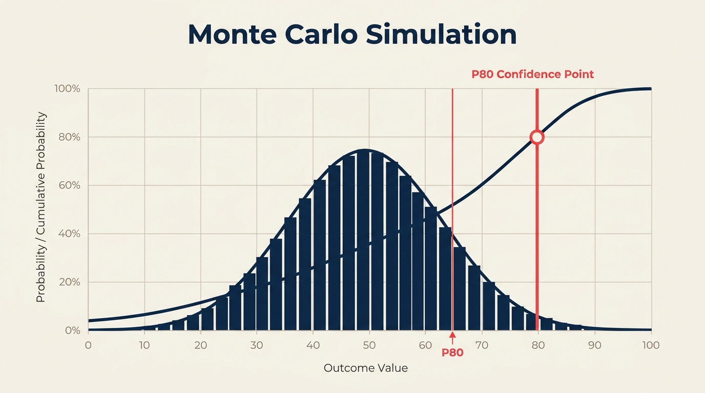
ステップ4:S字曲線を読み取り、P50とP80を特定する
出力は累積確率曲線です。最も重要なのは次の2点です。
- P50:シミュレーション試行の50%が完了した日付。統計的に偏りのない中央値の完了日です。
- P80:試行の80%が完了した日付。80%の確信度でコミットできる日付です。
多くのチームは、社内の計画目標としてP50を、外部のステークホルダーにコミットする日付としてP80を使用します。リスクの高いプロジェクトや契約上の縛りが強いプロジェクトでは、P85やP90を使うこともあります。
ステップ5:結果に基づいて行動する
P80の日付が契約上の締め切りより前であれば、スケジュールに余裕があります。P50の時点ですでに締め切りを超えているなら、構造的な問題を抱えています。今すぐスコープを削減する、リソースを追加する、あるいは期待値をリセットする必要があります。契約が遅延納品にペナルティを課す場合、P50の日付で交渉してはいけません。P80を使って交渉しましょう。
シミュレーションの出力を使って、どのタスクがスケジュールのばらつきに最も寄与しているかを特定しましょう。これらは、プロジェクトリスクマネジメント計画においてリスク軽減の対応が必要なタスクであり、リスクマトリクス上でも可視化すべきものです。
モンテカルロシミュレーションのメリット
現実的な予測。 シミュレーションは、マネージャーの楽観的な単一見積もりではなく、あり得る結果の全範囲を考慮します。相互に依存するタスクが多いプロジェクトは、並行パスが合流し最も長いパスが支配的になる「マージバイアス」の影響を特に受けやすくなります。単一値見積もりはこれを見逃しがちです。
ステークホルダーとのより良い対話。 P80の日付とS字曲線を提示することは、単一の日付を示すよりも誠実で、説明のしやすいアプローチです。確率を理解しているステークホルダーは、許容できるリスクについて情報に基づいた判断ができます。
リスクエクスポージャーの定量化。 分布の広がりは、どれだけの不確実性が存在するかを示します。分布が狭ければ、プロジェクトはよく理解されているということです。分布が広ければ、さらなる調査が必要というシグナルです。
優先度に基づくリスクマネジメント。 シミュレーションは、どのタスクがばらつきに最も寄与しているかを特定するため、リスク登録簿と軽減策の予算を正しい対象に集中させられます。
契約交渉を後押しする。 多くの大規模インフラプロジェクトや防衛プログラムでは、今や確率的なスケジュール分析が求められています。モンテカルロシミュレーションはその標準的な手法です。
よくある間違い
質の低い見積もり。 モンテカルロシミュレーションの精度は、投入する分布の質に左右されます。気まずい対話を避けるために悲観値を圧縮する(P = M + 20%など)チームは、一見精密に見えるものの統計的には誤った出力を生み出します。悲観的な見積もりは、多少悪いケースではなく、もっともらしい最悪のケースを反映すべきです。
タスク間の相関を無視する。 同じリソースが3つのタスクにまたがるボトルネックとなっているために一つのタスクが遅れる場合、3つすべてが一緒に遅れます。基本的なモンテカルロシミュレーションの多くはタスクを独立したものとして扱います。正の相関(一つの遅延が他の遅延を引き起こす傾向)をモデル化できていないと、スケジュールリスクを体系的に過小評価してしまいます。
P50を安全なコミットメントとして扱う。 P50は、遅れる確率が50%あるという意味です。それはコイントスと同じです。定時納品を期待するステークホルダーにP50の日付をコミットするのは、定期的な失望を招くレシピです。コミットメントにはP80以上を使いましょう。
シミュレーションを一度しか実行しない。 プロジェクトが進むにつれて入力は変化します。重要なマイルストーンや大きなリスクが顕在化したタイミングでシミュレーションを再実行しましょう。キックオフ時に一度だけ実行し、その後見直されないシミュレーションは、誤った安心感を与えるだけです。
S字曲線を読み違える。 P80の日付は「最悪のケース」ではありません。試行の80%が完了した時点にすぎません。それより後に完了する確率はまだ20%残っており、分布に長い裾があれば、かなり後になることもあります。
モンテカルロシミュレーションの例:ソフトウェアリリースプロジェクト
あるソフトウェアチームが、4つの主要フェーズからなる製品リリースを計画しています。三点見積もりは次の通りです。
| フェーズ | 楽観値 | 最頻値 | 悲観値 |
|---|---|---|---|
| アーキテクチャと設計 | 8日 | 12日 | 25日 |
| バックエンド開発 | 20日 | 30日 | 55日 |
| フロントエンドと統合 | 15日 | 22日 | 40日 |
| QAとリリース準備 | 6日 | 10日 | 20日 |
最頻値を使った単純な単一値見積もりでは、合計74日となります。チームはプロジェクト開始から80日後を締め切りとし、余裕があると感じています。
10,000回の反復によるモンテカルロシミュレーションを実行すると、結果はまったく異なるものになります。
| 確信度 | 完了までの期間 |
|---|---|
| P50 | 83日 |
| P70 | 91日 |
| P80 | 97日 |
| P90 | 108日 |
P50の時点ですでに80日という目標を超えています。80日以内に完了する確率はおよそ30%にとどまり、外部へのリリースコミットメントとして許容できる確信度の水準を大きく下回っています。チームは今や、スコープを圧縮する、バックエンドフェーズ(最もばらつきの大きいタスク)にリソースを追加する、あるいはリリース日を再交渉するかの明確な根拠を手にしています。シミュレーションの実行によって、単一値見積もりでは完全に見えなかった問題が明らかになったのです。
よくある質問
モンテカルロシミュレーションは何回反復すべきですか?
多くのプロジェクトスケジュールでは、1,000回の反復で使える分布が得られます。5,000回であれば、通常のレポーティングに十分な安定した結果が得られます。10,000回は、裾野の確率が重要となる、リスクの高いプロジェクトや契約上の分析における標準です。現代のソフトウェアでは反復回数を増やしてもコストはかからないため、5,000〜10,000回をデフォルトにするのは安全な習慣です。
P80の日付とは何ですか?
P80の日付とは、シミュレーション試行の80%が完了したプロジェクト完了日のことです。つまり、タスクの見積もりとその不確実性の範囲を踏まえると、その日付までにプロジェクトが完了する確率が80%あるという意味です。多くのプロジェクトマネジメント基準では、外部へのコミットメントには「確信度のある日付」としてP80を報告し、P50は社内チームの目標として使うことを推奨しています。
プロジェクトスケジュールのモンテカルロシミュレーションにはどのようなツールが使われますか?
一般的なツールには、Oracle Primavera Risk Analysis(旧Pertmaster)、Excel向けのPalisade @Risk、Oracle Crystal Ball、Safran Risk、Deltek Acumen Riskなどがあります。より軽量な用途では、PythonのライブラリであるNumPyやSciPyを使って独自のシミュレーションを構築するチームもあります。Microsoft Projectにはネイティブのモンテカルロ機能はありませんが、複数のアドインが連携できます。
モンテカルロシミュレーションとPERTの違いは何ですか?
どちらも三点見積もり(楽観値、最頻値、悲観値)を使用します。PERTは数式を使って単一の期待期間と標準偏差を計算し、一つの答えを導き出します。モンテカルロシミュレーションは何千回もの反復を実行し、PERTの数式では捉えられないマージバイアスを含む、タスク間の非線形な相互作用を反映した完全な確率分布を生み出します。並行パスの多い複雑なプロジェクトでは、モンテカルロシミュレーションの方が大幅に精度が高くなります。
モンテカルロシミュレーションはコスト予測にも使えますか?
はい。同じ手法をコストにも適用できます。タスクの期間の代わりに、費目やワークパッケージにコスト分布(楽観値、最頻値、悲観値)を割り当てます。シミュレーションはP50、P80、P90の値を伴うコスト確率分布を生み出し、恣意的なパーセンテージではなく、明確な確信度の水準に基づいてコンティンジェンシー予備費を設定できるようにします。
単一の締め切りと確率分布との間にあるギャップは、誤った安心感と情報に基づいたコミットメントとの間にあるギャップです。モンテカルロシミュレーションはプロジェクトの不確実性を減らすわけではありません。不確実性を目に見える形にすることで、適切なタスクにバッファを設け、誠実な締め切りを交渉し、一律10%のバッファを追加してうまくいくことを願うのではなく、実際のリスクの発生源に対応した軽減計画を立てられるようにします。
まずはばらつきが最も大きいタスクから着手し、悲観的な見積もりを誠実に校正した上で、少なくとも5,000回の反復を実行しましょう。そこで得られるS字曲線は、どんなガントチャートよりも、あなたのプロジェクトが抱える実際のスケジュールリスクについて多くを教えてくれるはずです。

Senior Operations & Growth Strategist
On this page
- モンテカルロシミュレーションとは
- モンテカルロシミュレーションの仕組み
- 三点見積もりの入力例
- モンテカルロシミュレーションと単一値見積もりの違い
- モンテカルロシミュレーションの実施方法
- ステップ1:プロジェクトネットワークをマッピングする
- ステップ2:すべてのタスクに三点見積もりを割り当てる
- ステップ3:シミュレーションを実行する
- ステップ4:S字曲線を読み取り、P50とP80を特定する
- ステップ5:結果に基づいて行動する
- モンテカルロシミュレーションのメリット
- よくある間違い
- モンテカルロシミュレーションの例:ソフトウェアリリースプロジェクト
- よくある質問
- モンテカルロシミュレーションは何回反復すべきですか?
- P80の日付とは何ですか?
- プロジェクトスケジュールのモンテカルロシミュレーションにはどのようなツールが使われますか?
- モンテカルロシミュレーションとPERTの違いは何ですか?
- モンテカルロシミュレーションはコスト予測にも使えますか?